Install Necesary Packages

 pkgs <-c(‘twitteR’,‘ROAuth’,‘httr’,‘plyr’,‘stringr’,‘ggplot2’,‘plotly’, ‘dplyr’) 
 for(p in pkgs) if(p %in% rownames(installed.packages()) == FALSE) {install.packages(p)}
 for(p in pkgs) suppressPackageStartupMessages(library(p, quietly=TRUE, character.only=TRUE))

Twitter Authorization

 # Set API Keys (Enter your credentials)
 api_key <- “#########################”				 
 api_secret <- “##################################################”					
 access_token <- “##################################################”					
 access_token_secret <- “#############################################”
 
 # Autorize Twitter
 library(twitteR)
 setup_twitter_oauth(api_key, api_secret, access_token, access_token_secret)

Sentiment Score Function

 score.sentiment <- function(sentences, good_text, bad_text, .progress=‘none’){ 
	require(plyr) 
	require(stringr) 
	 
	scores = laply(sentences, function(sentence, good_text, bad_text) {
	
		# clean up sentences with R's regex-driven global substitute, gsub():
		sentence = gsub('[[:punct:]]', '', sentence)
		sentence = gsub('[[:cntrl:]]', '', sentence)
		sentence = gsub('\\d+', '', sentence)
		#to remove emojis
		sentence <- iconv(sentence, 'UTF-8', 'ASCII')
		sentence = tolower(sentence)
		# split into words. str_split is in the stringr package
		word.list = str_split(sentence, '\\s+')
		# sometimes a list() is one level of hierarchy too much
		words = unlist(word.list)

		# compare our words to the dictionaries of positive & negative terms
		pos.matches = match(words, good_text)
		neg.matches = match(words, bad_text)

		# match() returns the position of the matched term or NA
		# we just want a TRUE/FALSE:
		pos.matches = !is.na(pos.matches)
		neg.matches = !is.na(neg.matches)

		# and conveniently enough, TRUE/FALSE will be treated as 1/0 by sum():
		score = sum(pos.matches) - sum(neg.matches)

		return(score)

	}, good_text, bad_text, .progress=.progress )
	
	scores.df = data.frame(score=scores, text=sentences) 
	return(scores.df)
	
 }

Brand Score Function

 brand.score <- function(brand.name, brand_tweet_text, positive_words = c(), negative_words = c()){
 
	require(twitteR)
	#Extract all brand tweets
	brand.tweets = searchTwitter(paste(brand_tweet_text, " exclude:retweets“), n=1000, lang=”en“, resultType =”recent“)
	
	#Convert all brand tweets in dataframe 
	brand.df <- twListToDF(brand.tweets)
	
	# Read in dictionary of positive and negative words
	positive.dict = scan(‘opinion-lexicon-English/positive-words.txt’, what=‘character’, comment.char=‘;’) 
	negative.dict = scan(‘opinion-lexicon-English/negative-words.txt’, what=‘character’, comment.char=‘;’) 
	
	# Add a few twitter-specific phrases 
	negative.text = c(negative.dict, negative_words)
	positive.text = c(positive.dict, positive_words)
	
	# Call the function and return a data frame 
	brand.sentiment <- score.sentiment(brand.df$text, positive.text, negative.text, .progress=‘text’)
	
	brand.sentiment$name <- brand.name
	return(brand.sentiment) 
 }

The Scores For Each Brand

 brand1.score <- brand.score(“united”, brand_tweet_text = "@united")
 brand2.score <- brand.score(“AmericanAir”, brand_tweet_text = "@AmericanAir") 
 brand3.score <- brand.score(“Delta”, brand_tweet_text = "@Delta") 
 brand4.score <- brand.score(“SouthwestAir”, brand_tweet_text = "@SouthwestAir") 
 brand5.score <- brand.score(“JetBlue”, brand_tweet_text = "@JetBlue")
 

Combine The Scores of All The Brands

 #Combine the scores of all the brand together
 all.brand.score <- rbind.fill(brand1.score, brand2.score, brand3.score, brand4.score, brand5.score)
 
 #Create a new data frame, Keeping back for future use
 brand.data <- all.brand.score

Clean the Brand Score Data

 #Remove the twitter text field
 brand.data <- brand.data[c(“name”, “score”)]
 
 #Remove all rows with neutral text i.e. values of 0
 brand.data <- brand.data[!brand.data$score == 0, ]
 
 #Consolidate and focus on all rows with value in between (-3,3)
 
 brand.data <- brand.data[!brand.data$score > 3, ]
 brand.data <- brand.data[!brand.data$score < (-3), ]

Plotting function

 brand.graph <- function(data.df, graph.color, industry.name){ 
 
	 require(ggplot2) 
	 
	 brand.plot <- data.df %>% 
		 ggplot(aes(x = score, fill = name)) + 
		 geom_histogram(binwidth = 1) + 
		 scale_fill_manual(values = graph.color) + 
		 theme_classic(base_size = 12) + 
		 scale_x_continuous(name = “Sentiment Score”) +
		 scale_y_continuous(name = “Tweets Counts”) +
		 ggtitle(paste(industry.name, “Twitter Sentiment on”, Sys.Date())) 
		 theme(axis.title.y = element_text(face=“bold”, colour=“#000000”, size=10), 
			 axis.title.x = element_text(face=“bold”, colour=“#000000”, size=8), 
			 axis.text.x = element_text(angle=16, vjust=0, size=8))
	 
	 return(brand.plot) 
 }

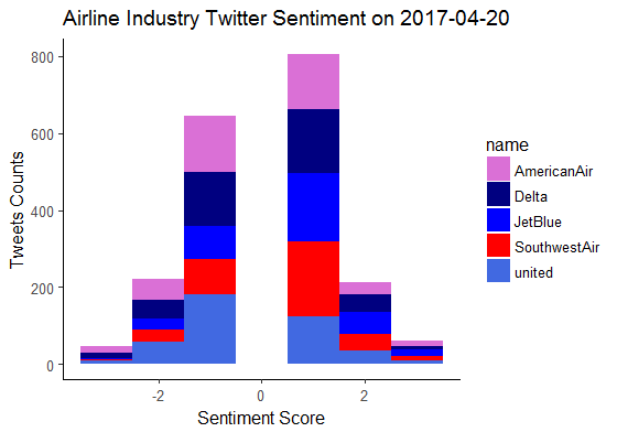
Plot the Scores of All Brands

 graph.color <- c(“orchid”,“navyblue”, “blue”, “red”, “royalblue”) 
 ep <- brand.graph(brand.data, graph.color, “Airline Industry”) 

 ep

Brand Score Graph

Summary